Bayesian regression with SGLD

This example shows how to use the SGLD sampler for a simple one-dimensional regression problem.

The full code is downloadable at the end of this page.

Imports

The following imports are needed to run this example.

import torch
import torch.nn as nn
from torch.utils.data import TensorDataset, DataLoader

from batorch.rkhs.discrepancies import KSD
from batorch.utils.misc import parameters_to_vector, vector_to_parameters
from batorch.likelihoods.regression_negloglike import GaussianNLL
from batorch.priordists.normal import Normal

from batorch.sgmcmc.samplers import SamplerSGLD
from batorch.rkhs.quantization import QuantizationMMD

from tqdm import tqdm

device = torch.device("cpu")

torch.manual_seed(0)

Prepare data

We first start by defining helpers for generating data and retrieving the network.

def get_model():
    return nn.Sequential(nn.Linear(1,50), nn.Tanh(), nn.Linear(50,50), nn.Tanh(), nn.Linear(50,1))

def prepare_data(sig_noise: float):
    f = lambda x: torch.cos(2.0*x) + torch.sin(x)

    x_train = 4*torch.rand((50,1))-2
    y_train = f(x_train) + torch.randn(*x_train.shape)*sig_noise**2

    x_test = torch.linspace(-3,3,200).view((-1,1))
    y_test = f(x_test)

    return (x_train, y_train), (x_test, y_test)

Datasets and Dataloaders

Instantiate datasets and dataloaders as you would do in a typical training pipeline with PyTorch.

# Prepare data
sig_noise = 0.3
(x_train, y_train), (x_test, y_test) = prepare_data(sig_noise)

train_dataset, test_dataset = TensorDataset(x_train, y_train), TensorDataset(x_test, y_test)
train_loader, test_loader = DataLoader(dataset=train_dataset, batch_size=32, shuffle=True), DataLoader(dataset=test_dataset, batch_size=32, shuffle=False)

Posterior distribution

The next step consists in defining the negative log-loglikelihood and the negative log-prior. Here, we use a simple feed-forward neural network as a surrogate model, a homoscedastic Gaussian likelihood, and a normal prior.

Note that the negative log-loglikelihood is a torch.nn.Module and the negative log-prior is a torch.distrubtion.Distribution object.

surrogate_model = get_model()
nll = GaussianNLL(model=surrogate_model, variance_prior=sig_noise**2).to(device)
nlp = Normal(loc=0.0, scale=1.0).to(device)

Sampling

At this stage, we have all we need for using the SGLD sampler.

sampler = SamplerSGLD(negloglikelihood=nll, neglogprior=nlp, init_params=None, dataloader=train_loader, step_size=1e-5)

num_iter, num_burnin = 20000, 10000

samples = []
for iter in tqdm(range(num_iter), desc="Sampling with SGLD"):
    for _, (x, y) in enumerate(train_loader):
        x, y = x.to(device), y.to(device)
        loss = sampler.step(x, y)
    if iter > num_burnin:
        samples.append(sampler.get_params())
samples = torch.stack(samples,dim=0)

Quantization

Before making predictions, we select a few samples by minimizing the maximum mean discrepancy.

Here we also specify that we would like to perform the quantization on a GPU if one is available.

thinner = QuantizationMMD(m=2000)
idx = thinner.select({"samples": samples}, memory_is_bottleneck=False, device=torch.device("cuda" if torch.cuda.is_available() else "cpu"))
subsamples = torch.stack([samples[i] for i in idx],dim=0)

Predict

We then use the selected samples for making predictions with the surrogate model.

predictions = []
with torch.no_grad():
    surrogate_model.eval()

    for i in tqdm(range(len(subsamples)), desc="Predicting"):
        vector_to_parameters(subsamples[i], surrogate_model.parameters(), grad=False)

        predictions_i = []
        for _, (x, y) in enumerate(test_loader):
            x, y = x.to(device), y.to(device)
            prediction_batch = surrogate_model(x)
            predictions_i.append(prediction_batch)
        predictions_i = torch.concat(predictions_i, dim=0)
        predictions.append(predictions_i)

    predictions = torch.stack(predictions,dim=0).cpu().detach().numpy().squeeze()

Kernelized Stein discrepancy

Optionally, we can also compute the kernelized Stein discrepancy in order to evaluate the quality of the posterior approximation.

For this, we need to compute the full-batch logarithm of the posterior distribution.

grads = torch.zeros_like(subsamples)
for i in range(len(subsamples)):
    vector_to_parameters(samples[i], nll.parameters(), grad=False)
    nll.zero_grad()
    for batch_idx, (x, y) in enumerate(train_loader):
        x, y = x.to(device), y.to(device)
        negloglike = nll(x, y)
        if batch_idx==0:
            neglogprior = nlp(nll.parameters())
            neglogpost = negloglike + neglogprior
        else:
            neglogpost = negloglike
        neglogpost.backward()
    grads[i] = parameters_to_vector(nll.parameters(), grad=True, both=False)
grads.mul_(-1.0)

Then we simply call the function that estimates the KSD with a V-statistics:

ksd = KSD(x=subsamples, grad_x=grads)

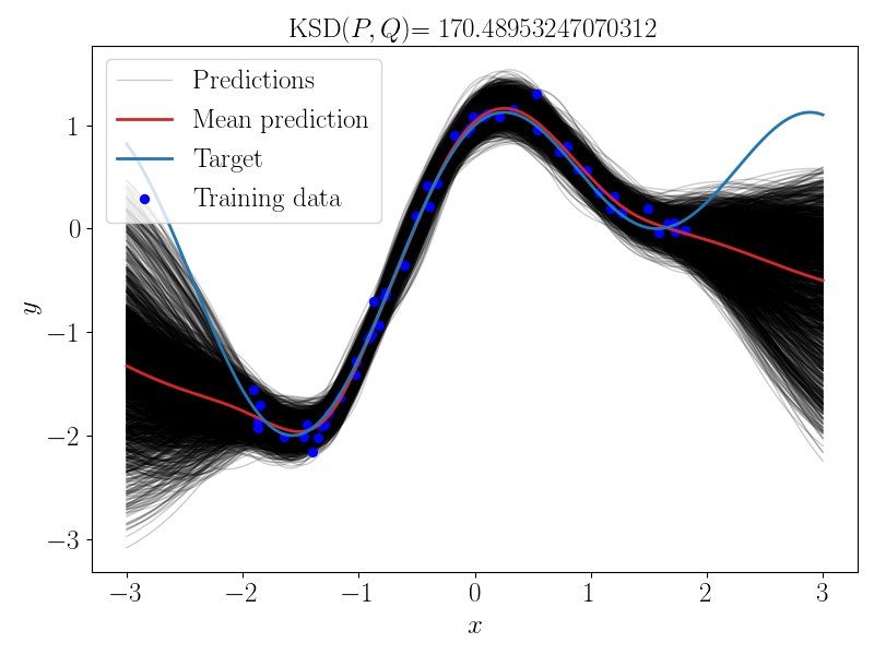
Bayesian neural network predictions

The full example that reproduces this figure is shown below.

Full example script

batorch_tutorial.py

import torch
import torch.nn as nn
from torch.utils.data import TensorDataset, DataLoader

from batorch.rkhs.discrepancies import KSD
from batorch.utils.misc import parameters_to_vector, vector_to_parameters
from batorch.likelihoods.regression_negloglike import GaussianNLL
from batorch.priordists.normal import Normal

from batorch.sgmcmc.samplers import SamplerSGLD
from batorch.rkhs.quantization import QuantizationMMD

from tqdm import tqdm

def get_model():
    return nn.Sequential(nn.Linear(1,50), nn.Tanh(), nn.Linear(50,50), nn.Tanh(), nn.Linear(50,1))

def prepare_data(sig_noise: float):
    f = lambda x: torch.cos(2.0*x) + torch.sin(x)

    x_train = 4*torch.rand((50,1))-2
    y_train = f(x_train) + torch.randn(*x_train.shape)*sig_noise**2

    x_test = torch.linspace(-3,3,200).view((-1,1))
    y_test = f(x_test)

    return (x_train, y_train), (x_test, y_test)

if __name__ == "__main__":

    # Pick a device
    device = torch.device("cpu")
    torch.manual_seed(0)

    # Prepare data
    sig_noise = 0.3
    (x_train, y_train), (x_test, y_test) = prepare_data(sig_noise)

    train_dataset, test_dataset = TensorDataset(x_train, y_train), TensorDataset(x_test, y_test)
    train_loader, test_loader = DataLoader(dataset=train_dataset, batch_size=32, shuffle=True), DataLoader(dataset=test_dataset, batch_size=32, shuffle=False)

    # Define log-target
    surrogate_model = get_model()
    nll = GaussianNLL(model=surrogate_model, variance_prior=sig_noise**2).to(device)
    nlp = Normal(loc=0.0, scale=1.0).to(device)

    # Sample with SGLD
    sampler = SamplerSGLD(negloglikelihood=nll, neglogprior=nlp, init_params=None, dataloader=train_loader, step_size=1e-5)

    num_iter, num_burnin = 20000, 10000

    samples = []
    for iter in tqdm(range(num_iter), desc="Sampling with SGLD"):
        for _, (x, y) in enumerate(train_loader):
            x, y = x.to(device), y.to(device)
            loss = sampler.step(x, y)
        if iter > num_burnin:
            samples.append(sampler.get_params())
    samples = torch.stack(samples,dim=0)

    # Thinning
    thinner = QuantizationMMD(m=2000)
    idx = thinner.select({"samples": samples}, memory_is_bottleneck=False, device=torch.device("cuda" if torch.cuda.is_available() else "cpu"))
    subsamples = torch.stack([samples[i] for i in idx],dim=0)

    # Predict
    predictions = []
    with torch.no_grad():
        surrogate_model.eval()

        for i in tqdm(range(len(subsamples)), desc="Predicting"):
            vector_to_parameters(subsamples[i], surrogate_model.parameters(), grad=False)

            predictions_i = []
            for _, (x, y) in enumerate(test_loader):
                x, y = x.to(device), y.to(device)
                prediction_batch = surrogate_model(x)
                predictions_i.append(prediction_batch)
            predictions_i = torch.concat(predictions_i, dim=0)
            predictions.append(predictions_i)

        predictions = torch.stack(predictions,dim=0).cpu().detach().numpy().squeeze()

    # Computing the kernelized Stein discrepancy
    grads = torch.zeros_like(subsamples)
    for i in range(len(subsamples)):
        vector_to_parameters(samples[i], nll.parameters(), grad=False)
        nll.zero_grad()
        for batch_idx, (x, y) in enumerate(train_loader):
            x, y = x.to(device), y.to(device)
            negloglike = nll(x, y)
            if batch_idx==0:
                neglogprior = nlp(nll.parameters())
                neglogpost = negloglike + neglogprior
            else:
                neglogpost = negloglike
            neglogpost.backward()
        grads[i] = parameters_to_vector(nll.parameters(), grad=True, both=False)
    grads.mul_(-1.0)
    ksd = KSD(x=subsamples, grad_x=grads)

    # Plot the results
    import matplotlib.pyplot as plt
    plt.rcParams.update({
    "text.usetex": True,
    "font.family": "sans-serif",
    "font.sans-serif": ["Helvetica"]})
    fig, ax = plt.subplots(1,1,figsize=(8,6))
    ax.plot(x_test, predictions.T, linestyle="-", linewidth=1, color="k", alpha=0.2, zorder=-1)
    ax.plot(x_test, predictions[0], linestyle="-", linewidth=1, color="k", alpha=0.2, label=r"$\mathrm{Predictions}$", zorder=-1)
    ax.plot(x_test, predictions.mean(axis=0), linestyle="-", linewidth=2, color="tab:red", label=r"$\mathrm{Mean}$ $\mathrm{prediction}$")
    ax.plot(x_test, y_test, linestyle="-", linewidth=2, color="tab:blue", label=r"$\mathrm{Target}$")
    ax.scatter(x_train, y_train, color="b", marker="o", s=32, label=r"$\mathrm{Training}$ $\mathrm{data}$")
    ax.set_xlabel(r"$x$", fontsize=18)
    ax.set_ylabel(r"$y$", fontsize=18)
    ax.set_title(r"$\mathrm{KSD}(P,Q)$" + rf"$ = {ksd}$", fontsize=18)
    ax.legend(fontsize=18)
    ax.tick_params(labelsize=18)
    fig.tight_layout()
    plt.savefig("batorch_tutorial.png", format="png")